Orthogonality, eigen/SVD/condition number, effective rank — each with a runnable demo. Optional: read it when a foundations module points here.
1. Orthogonality & orthonormality
The inner product\(\mathbf u^\top\mathbf v=\sum_i u_i v_i=\lVert\mathbf u\rVert\lVert\mathbf v\rVert\cos\theta\) measures alignment. Two non-zero vectors are orthogonal (\(\mathbf u\perp\mathbf v\)) when \(\mathbf u^\top\mathbf v=0\) — i.e. \(\theta=90^\circ\), no shared component. A set is orthonormal when every pair is orthogonal and each vector has unit length. An orthonormal basis is the nicest coordinate system there is: every vector decomposes as \(\mathbf x=\sum_i(\mathbf q_i^\top\mathbf x)\,\mathbf q_i\), and writing along one \(\mathbf q_i\) leaves all the others untouched.
Why the course cares. An associative memory stores \(\mathcal M=\sum_i\mathbf v_i\mathbf k_i^\top\) and reads with \(\mathcal M\mathbf k_j=\sum_i\mathbf v_i(\mathbf k_i^\top\mathbf k_j)\). If the keys are orthonormal, every cross term \(\mathbf k_i^\top\mathbf k_j\) (\(i\neq j\)) is \(0\) and you get back exactly \(\mathbf v_j\) — perfect recall. The moment keys overlap, those cross terms leak other values into the answer: crosstalk.
import numpy as npnp.random.seed(0)d, N =8, 8# orthonormal keys (columns of a random orthogonal matrix) vs correlated keys (clustered)Q = np.linalg.qr(np.random.randn(d, d))[0]keys_on = Q[:, :N]base = np.random.randn(d); base /= np.linalg.norm(base)keys_corr = np.stack([(lambda k: k/np.linalg.norm(k))(base +0.6*np.random.randn(d)) for _ inrange(N)], 1)vals = np.random.randn(N, d)def recall_err(K): M =sum(np.outer(vals[i], K[:, i]) for i inrange(N)) # M = Σ vᵢ kᵢᵀreturn np.mean([np.linalg.norm(M @ K[:, i] - vals[i]) for i inrange(N)])def max_offdiag(K): G = np.abs(K.T @ K); np.fill_diagonal(G, 0);return G.max() # largest |kᵢ·kⱼ|, i≠jprint(f"orthonormal keys : max |kᵢ·kⱼ| = {max_offdiag(keys_on):.3f} mean recall err = {recall_err(keys_on):.4f}")print(f"correlated keys : max |kᵢ·kⱼ| = {max_offdiag(keys_corr):.3f} mean recall err = {recall_err(keys_corr):.4f}")print("→ orthonormal: zero cross terms → perfect recall. correlated: cross terms leak → crosstalk.")
orthonormal keys : max |kᵢ·kⱼ| = 0.000   mean recall err = 0.0000
correlated keys  : max |kᵢ·kⱼ| = 0.866   mean recall err = 2.9458
→ orthonormal: zero cross terms → perfect recall.  correlated: cross terms leak → crosstalk.
The same fact, stated for writing: storing a new association along a direction orthogonal to an old one does not disturb the old readout. Overlap is exactly what causes interference — and, one level up, what makes “orthogonal tasks” the hardest case for an optimizer’s memory (M6 §2.1).
import numpy as npnp.random.seed(0)d =8Q = np.linalg.qr(np.random.randn(d, d))[0]k1 = Q[:, 0]v1, v2 = np.random.randn(d), np.random.randn(d)for name, k2 in [("k2 ⟂ k1", Q[:, 1]), ("k2 overlaps k1", (k1 +0.5* Q[:, 2]) / np.linalg.norm(k1 +0.5* Q[:, 2]))]: M = np.outer(v1, k1) + np.outer(v2, k2) # store v1@k1, then also v2@k2print(f"{name:<16}: cos(k1,k2)={k1 @ k2:+.2f} ‖readout(k1) − v1‖ = {np.linalg.norm(M @ k1 - v1):.4f}")print("→ an orthogonal second write is invisible to the first key; an overlapping one corrupts it.")
k2 ⟂ k1         : cos(k1,k2)=+0.00   ‖readout(k1) − v1‖ = 0.0000
k2 overlaps k1  : cos(k1,k2)=+0.89   ‖readout(k1) − v1‖ = 1.9282
→ an orthogonal second write is invisible to the first key; an overlapping one corrupts it.
2. Eigenvalues, SVD, and the condition number
A matrix stretches space by different amounts along different directions.
For a symmetric matrix \(A\) (e.g. a curvature/Hessian), the eigen-decomposition\(A=\sum_i\lambda_i\mathbf q_i\mathbf q_i^\top\) gives orthonormal directions \(\mathbf q_i\) each scaled by an eigenvalue \(\lambda_i\).
For a general matrix \(M\), the SVD\(M=U\Sigma V^\top\) does the same with singular values\(\sigma_i\ge0\) (the \(\sigma_i\) are the square roots of the eigenvalues of \(M^\top M\)).
The condition number\(\kappa=\sigma_{\max}/\sigma_{\min}\) (or \(\lambda_{\max}/\lambda_{\min}\)) measures how lopsided the stretch is. \(\kappa=1\) = stretches everything equally (a sphere stays a sphere); large \(\kappa\) = a long thin ellipse.
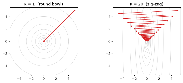
Where this bites in the course. On a quadratic loss \(\tfrac12\mathbf w^\top A\mathbf w\), gradient descent must keep its step size safe for the steepest direction (\(\lambda_{\max}\)), so it crawls along the flattest one (\(\lambda_{\min}\)): its convergence rate is \(\tfrac{\kappa-1}{\kappa+1}\), which \(\to1\) (no progress) as \(\kappa\) grows. That is the zig-zag, and it is the problem momentum and preconditioning exist to fix (M6).
import numpy as np, matplotlib.pyplot as pltdef gd_path(kappa, steps, th=1e-12): A = np.diag([kappa, 1.0]) w = np.array([5.0, 5.0]) lr =2/ (kappa +1) path = [w.copy()] n =Nonefor t inrange(steps): w = w - lr * (A @ w) path.append(w.copy())if n isNoneand0.5* w @ A @ w <1e-8: n = t +1return np.array(path), nfor kappa in [1.0, 20.0, 100.0]: _, n = gd_path(kappa, 2000)print(f"κ={kappa:>5}: rate (κ-1)/(κ+1) = {(kappa -1) / (kappa +1):.3f} steps to loss<1e-8 = {n}")# visualize the zig-zag: ill-conditioned (κ=20) vs round bowl (κ=1)fig, axes = plt.subplots(1, 2, figsize=(9, 3.6))for ax, kappa inzip(axes, [1.0, 20.0]): A = np.diag([kappa, 1.0]) path, _ = gd_path(kappa, 40) xs = np.linspace(-5.5, 5.5, 200) ys = np.linspace(-5.5, 5.5, 200) X, Y = np.meshgrid(xs, ys) Z =0.5* (kappa * X**2+ Y**2) ax.contour(X, Y, Z, levels=np.logspace(-1, 2.5, 12), colors="lightgray", linewidths=0.7) ax.plot(path[:, 0], path[:, 1], "-o", ms=3, lw=1, color="C3") ax.set_title(f"κ = {kappa:g}"+ (" (round bowl)"if kappa ==1else" (zig-zag)")) ax.set_aspect("equal")plt.tight_layout()plt.show()
Whitening / orthogonalization. Many fixes amount to reshaping the ellipse back into a sphere — mapping all singular values toward \(1\), i.e. driving \(\kappa\to1\). Adam and Newton do it with a preconditioner; Muon / Atlas do it directly on a matrix with the Newton–Schulz iteration, an approximate orthogonalization that pushes every \(\sigma_i\to1\) without ever forming the SVD (NL-1 §Atlas, M6 §4).
import numpy as npnp.random.seed(0)M = np.random.randn(6, 6)sv = np.linalg.svd(M, compute_uv=False)print(f"singular values : {np.round(sv, 3)}")print(f"condition number κ : {sv.max() / sv.min():.2f}")def newton_schulz(G, k=5): # approximate orthogonalization (no SVD) a, b, c =3.4445, -4.7750, 2.0315 X = G / np.linalg.norm(G)for _ inrange(k): AX = X @ X.T X = a * X + b * (AX @ X) + c * (AX @ AX @ X)return Xsw = np.linalg.svd(newton_schulz(M), compute_uv=False)print(f"after Newton–Schulz: σ ∈ [{sw.min():.3f}, {sw.max():.3f}] κ = {sw.max() / sw.min():.2f} (≈ 1 → ~orthogonal)")
The rank of a matrix is the number of independent directions its columns span. But for a memory, the binary “independent or not” is too crude — two keys at \(1°\) apart are technically independent yet practically the same direction. What matters is the effective rank: how many directions are meaningfully used. A convenient measure is the participation ratio of the singular values,
which equals the true count when directions are balanced (orthonormal) and collapses toward \(1\) as they pile onto one axis.
Why the course cares. This is associative-memory capacity (M1, M2): you can store cleanly about as many associations as the effective rank of the key set — not the nominal matrix rank. Below, eight keys with full matrix-rank 8 but effective rank ~3 already overflow, exactly like eight near-parallel keys would.
import numpy as npnp.random.seed(0)d =8def eff_rank(K): s = np.linalg.svd(K, compute_uv=False) s2 = s**2return (s2.sum() **2) / (s2**2).sum()def recall_err(K, vals): N = K.shape[1] M =sum(np.outer(vals[i], K[:, i]) for i inrange(N))return np.mean([np.linalg.norm(M @ K[:, i] - vals[i]) for i inrange(N)])Q = np.linalg.qr(np.random.randn(d, d))[0]print(f"{'key set':<30}{'#keys':>6}{'matrix rank':>13}{'eff. rank':>11}{'recall err':>12}")for N in [4, 8]: # orthonormal, within capacity K = Q[:, :N] vals = np.random.randn(N, d)print(f"{'orthonormal (⟂)':<30}{N:>6}{np.linalg.matrix_rank(K):>13}{eff_rank(K):>11.2f}{recall_err(K, vals):>12.4f}" )base = np.random.randn(d)base /= np.linalg.norm(base) # correlated: full matrix-rank, low eff-rankK = np.stack([(lambda k: k / np.linalg.norm(k))(base +0.6* np.random.randn(d)) for _ inrange(8)], 1)print(f"{'correlated (clustered)':<30}{8:>6}{np.linalg.matrix_rank(K):>13}{eff_rank(K):>11.2f}{recall_err(K, np.random.randn(8, d)):>12.4f}")K = np.random.randn(d, 14)K /= np.linalg.norm(K, axis=0) # over capacity: N > dprint(f"{'random, OVER capacity (N>d)':<30}{14:>6}{np.linalg.matrix_rank(K):>13}{eff_rank(K):>11.2f}{recall_err(K, np.random.randn(14, d)):>12.4f}")print("\n→ clean recall tracks EFFECTIVE rank, not matrix rank: full-rank-but-correlated keys still overflow.")
M1 — Associative memory — orthonormal keys → clean recall; capacity ≈ effective rank of the key set (§1, §3).
M2 — Fast Weight Programmers — capacity law \(\approx d_{\text{key}}\) is the same effective-rank statement (§3).
M3 — Linear attention — the feature map \(\phi\) raises the effective dimension of the keys to buy capacity; softmax’s infinite-dim kernel is the orthogonality limit (§1, §3).
M6 — Optimizers as associative memories — ill-conditioning → zig-zag that momentum smooths (§2); orthogonal tasks = worst-case forgetting (§1); Muon = orthogonalizing the gradient; Adam/preconditioning drive \(\kappa\to1\).