NL-3 aside — a genuine multi-frequency Continuum Memory System

A companion to NL-3, built to answer one question: the HOPE-training aside used a block it called “CMS” — but that was a single Linear→GELU→Linear MLP updated once per training step, i.e. the degenerate \(k\)=1, single-frequency case (which is just a Transformer MLP, NL-2 §4). It had no continuum of frequencies. So what does the real thing look like? Optional.

Runs on CPU in seconds; pure PyTorch, no GPU.

This notebook builds it: a chain of memories that update in-context at genuinely different frequencies (NL Eq. 70–71, and the head-wise variant of Eq. 74), instrumented so you can see the levels.

The point to demonstrate concretely:

the levels update at different cadences — a fast level rewrites itself every step, a slow level only at chunk boundaries;
the fast level churns (large cumulative parameter movement) while the slow level stays nearly persistent;
the multi-frequency system works on a non-stationary task, and the continuum modestly beats any single frequency.

Grounding: NL §7.1 (CMS; Eq. 71’s chunked per-level update; Eq. 74’s head-wise variant). Builds on NL-2 (levels = update frequency) and NL-3 (HOPE).

1. What “multi-frequency” means here

A CMS is a set of memories \(\mathcal M^{(f_1)},\dots,\mathcal M^{(f_k)}\) at \(k\) different frequencies. In the head-wise variant (Eq. 74) they run on the same input and their outputs are combined, \(\mathbf y_t=\text{Agg}\big(\mathcal M^{(f_k)}(\mathbf x_t),\dots,\mathcal M^{(f_1)}(\mathbf x_t)\big)\) — the paper leaves \(\text{Agg}(\cdot)\) arbitrary and suggests a learnable weighted sum; we use a plain sum. Level \(\ell\)’s parameters update only every \(C^{(\ell)}\) steps, accumulating their update over the chunk and applying it at the boundary (Eq. 71). \(C^{(\ell)}=1\) is the fastest level (rewrites every step); a large \(C^{(\ell)}\) is a slow, persistent level.

We learn online on a non-stationary target — a linear map \(W\) that drifts a little every step — so there is genuinely something for a fast level to track and something for a slow level to stabilize. (We use a linear memory per level for clarity; the paper uses residual-MLP blocks — deep memories, NL-1 — but the frequency structure is identical.)

import numpy as np
import torch

torch.manual_seed(0)
d = 16


def run(periods, lr=0.5, T=600, drift=0.01, seed=1, record=False):
    gen = torch.Generator().manual_seed(seed)
    W = torch.randn(d, d, generator=gen) / np.sqrt(d)
    dW = torch.randn(d, d, generator=gen) / np.sqrt(d) * drift  # slow drift direction
    Ms = [torch.zeros(d, d) for _ in periods]
    acc = [torch.zeros(d, d) for _ in periods]
    cnt = [0] * len(periods)
    updates = [0] * len(periods)
    movement = [0.0] * len(periods)
    err_curve = []
    move_ts = [[] for _ in periods]  # per-level cumulative |Δθ| over time
    for t in range(T):
        W = W + dW  # target drifts (non-stationary)
        x = torch.randn(d, generator=gen)
        x /= x.norm()
        y = W @ x
        err = sum(M @ x for M in Ms) - y  # head-wise output (Eq. 74)
        err_curve.append(err.norm().item())
        for l, Cl in enumerate(periods):
            acc[l] += torch.outer(err, x)
            cnt[l] += 1  # accumulate this level's gradient
            if cnt[l] >= Cl:  # chunk boundary -> update level l (Eq. 71)
                upd = lr * acc[l] / cnt[l]
                Ms[l] = Ms[l] - upd
                movement[l] += upd.norm().item()
                acc[l] = torch.zeros(d, d)
                cnt[l] = 0
                updates[l] += 1
        if record:
            for l in range(len(periods)):
                move_ts[l].append(movement[l])
    return np.array(err_curve), updates, movement, move_ts


periods = [1, 10, 50]
err, updates, movement, move_ts = run(periods, record=True)
print(f"CMS with update periods C = {periods}  (level 0 fastest, level {len(periods) - 1} slowest)")
for l, Cl in enumerate(periods):
    print(f"  level {l}  (C={Cl:>2}):  {updates[l]:>3} updates over 600 steps,   cumulative |Δθ| = {movement[l]:.2f}")
print(f"\nmean tracking error over 2nd half: {err[300:].mean():.3f}")

CMS with update periods C = [1, 10, 50]  (level 0 fastest, level 2 slowest)
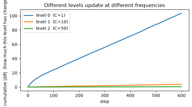
  level 0  (C= 1):  600 updates over 600 steps,   cumulative |Δθ| = 103.59
  level 1  (C=10):   60 updates over 600 steps,   cumulative |Δθ| = 3.83
  level 2  (C=50):   12 updates over 600 steps,   cumulative |Δθ| = 0.50

mean tracking error over 2nd half: 0.320

The levels are real. Read the counts: level 0 updates every step (600 updates) and its parameters move a lot (it is constantly rewriting itself to track the drift); level 2 updates only 12 times and barely moves — a slow, persistent store. Three genuinely different frequencies, exactly as NL-2 defines a level. Now plot the cumulative movement over time and the different cadences become a picture.

import matplotlib.pyplot as plt
plt.figure(figsize=(6.4, 3.6))
for l, Cl in enumerate(periods):
    plt.plot(move_ts[l], label=f"level {l}  (C={Cl})", lw=2)
plt.xlabel("step"); plt.ylabel("cumulative |Δθ|  (how much this level has changed)")
plt.title("Different levels update at different frequencies")
plt.legend(); plt.tight_layout(); plt.show()
print("fast level: smooth steady climb (updates every step).")
print("slow levels: flat plateaus broken by occasional steps (updates only at chunk boundaries).")

fast level: smooth steady climb (updates every step).
slow levels: flat plateaus broken by occasional steps (updates only at chunk boundaries).

2. Does the continuum help? — vs single frequencies

Compare the 3-level CMS against using only one frequency. On this fast-drifting target a single slow level can’t keep up; a single fast level does most of the work; and the continuum edges out the best single frequency by adding stable levels under the fast one.

print(f"{'config':>18}  {'mean tracking err (2nd half)':>28}  {'updates/level':>16}")
for name, P in [("fast only [1]", [1]), ("slow only [50]", [50]),
                ("CMS [1,50]", [1, 50]), ("CMS [1,10,50]", [1, 10, 50])]:
    e, u, m, _ = run(P)
    print(f"{name:>18}  {e[300:].mean():>28.3f}  {str(u):>16}")
print("\nslow-only can't track the drift; fast-only does most of the work;")
print("the continuum [1,10,50] is best — fast level tracks the drift, slower levels add a stable backbone.")

            config  mean tracking err (2nd half)     updates/level
     fast only [1]                         0.354             [600]
    slow only [50]                         4.049              [12]
        CMS [1,50]                         0.347         [600, 12]
     CMS [1,10,50]                         0.320     [600, 60, 12]

slow-only can't track the drift; fast-only does most of the work;
the continuum [1,10,50] is best — fast level tracks the drift, slower levels add a stable backbone.

What this shows — and the honest scope

This is a real continuum, not the \(k\)=1 MLP: three memories updating in-context at three different frequencies (Eq. 71), instrumented so you can see the fast level churn and the slow levels persist. That is precisely the “levels (frequencies)” that the HOPE-training aside’s block lacked.
It works and the continuum helps — on a non-stationary target the multi-frequency system tracks better than any single frequency, modestly.

Honest scope. The gain here is modest, and on a fast-drifting target the fast level does most of the work — adding levels is a small, consistent improvement, not a dramatic one. The large payoff CMS is built for — resisting catastrophic forgetting across many tasks over a long lifetime (§7.1) — is not something a small linear toy shows cleanly; it needs the full nonlinear, nested machinery, meta-learned initial states, and scale (the same caveat as NL-2 §4 and NL-3 §6). What this notebook does settle is the mechanical question: a genuine CMS has multiple levels at multiple frequencies, and here they are, measured.

Back-reference. In the HOPE-training aside the cms block is the degenerate \(k\)=1 case (one MLP, one frequency = a Transformer MLP). This notebook is the \(k\ge 2\) continuum it was standing in for.